

Double-Branch DenseNet-Transformer Hyperspectral Image Classification
-
摘要: 为了减少高光谱图像的训练样本,同时得到更好的分类结果,本文提出了一种基于密集连接网络和空谱变换器的双支路深度网络模型。该模型包含两个支路并行提取图像的空谱特征。首先,两支路分别使用3D和2D卷积对子图像的空间信息和光谱信息进行初步提取,然后经过由批归一化、Mish函数和3D卷积组成的密集连接网络进行深度特征提取。接着两支路分别使用光谱变换器和空间变换器以进一步增强网络提取特征的能力。最后两支路的输出特征图进行融合并得到最终的分类结果。模型在Indian Pines、University of Pavia、Salinas Valley和Kennedy Space Center数据集上进行了测试,并与6种现有方法进行了对比。结果表明,在Indian Pines数据集的训练集比例为3%,其他数据集的训练集比例为0.5%的条件下,算法的总体分类精度分别为95.75%、96.75%、95.63%和98.01%,总体性能优于比较的方法。Abstract: To reduce the training samples of hyperspectral images and obtain better classification results, a double-branch deep network model based on DenseNet and a spatial-spectral transformer was proposed in this study. The model includes two branches for extracting the spatial and spectral features of the images in parallel. First, the spatial and spectral information of the sub-images was initially extracted using 3D convolution in each branch. Then, the deep features were extracted through a DenseNet comprising batch normalization, mish function, and 3D convolution. Next, the two branches utilized the spectral transformer module and spatial transformer module to further enhance the feature extraction ability of the network. Finally, the output characteristic maps of the two branches were fused and the final classification results were obtained. The model was tested on Indian pine, University of Pavia, Salinas Valley, and Kennedy Space Center datasets, and its performance was compared with six types of current methods. The results demonstrate that the overall classification accuracies of our model are 95.75%, 96.75%, 95.63%, and 98.01%, respectively when the proportion of the training set of Indian pines is 3% and the proportion of the training set of the rest is 0.5%. The overall performance was better than that of other methods.
-

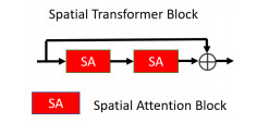
图 3 Spatial transformer block 原理
Figure 3. Spatial transformer block schematic diagram

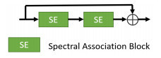
图 4 Spectral association block 原理
Figure 4. Spectral association block schematic diagram

图 5 Spectral transformer block 原理
Figure 5. Spectral transformer block schematic diagram

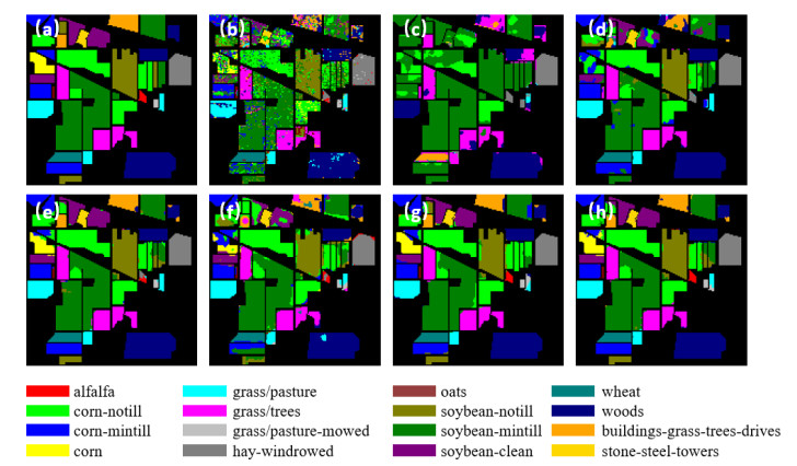
图 7 IP数据集的分类结果图(a)标签;(b)SVM;(c)CDCNN;(d)SSRN;(e)FDSSC;(f)DBMA;(g) DBDA;(h)Ours
Figure 7. Classification result diagram of the IP dataset (a) label; (b)SV; (c) CDCNN; (d) SSRN; (e) FDSSC; (f) DBMA; (g) DBDA; (h) Ours

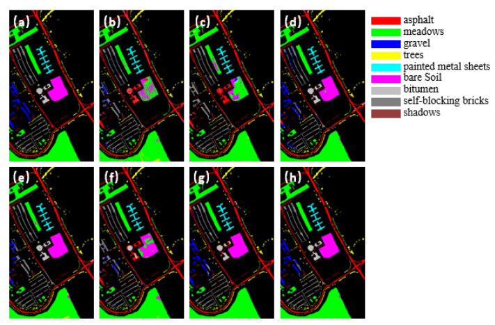
图 8 UP数据集的分类结果图(a)标签;(b)SVM;(c)CDCNN;(d)SSRN;(e)FDSSC;(f) DBMA;(g) DBDA;(h)Ours
Figure 8. Classification result diagram of the UP dataset (a) label; (b) SVM; (c) CDCNN; (d) SSRN; (e) FDSSC; (f) DBMA; (g) DBDA; (h) Ours

图 9 SV数据集的分类结果图(a)标签;(b)SVM;(c)CDCNN;(d)SSRN;(e)FDSSC;(f)DBMA;(g)DBDA;(h)Ours
Figure 9. Classification result diagram of the SV dataset. (a) label; (b) SVM; (c) CDCNN; (d) SSRN; (e) FDSSC; (f) DBMA; (g) DBDA; (h) Ours

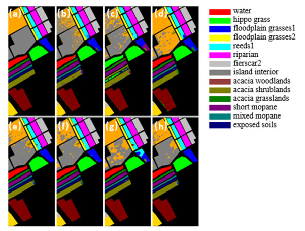
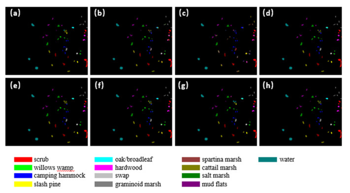
图 10 KSC数据集的分类结果图(a)标签;(b)SVM;(c)CDCNN;(d)SSRN;(e)FDSSC;(f)DBMA;(g)DBDA;(h)Ours
Figure 10. Classification result diagram of the KSC dataset (a) label; (b) SVM; (c) CDCNN; (d) SSRN; (e) FDSSC; (f) DBMA; (g) DBDA; (h) Ours
表 1 数据集参数
Table 1. Dataset parameters
Parameters Dataset IP UP SV KSC Acquisition time 2001 2003 1992 1996 Location A farm in northwestern Indiana, USA Part of Pavia, Italy Salinas Valley, California, USA Kennedy Space Center, Florida, USA Sensor AVIRIS ROSIS AVIRIS AVIRIS Resolution/m 20 1.3 3.7 18 Spectral range/μm [0.4, 2.5] [0.43, 0.86] [0.4, 2.5] [0.4, 2.5] Spectral band 200 103 204 176 Size/(pixel×pixel) 145×145 610×340 512×217 512×614 Land-cover 16 9 16 13 Total sample pixel 21025 42776 54129 5211  下载: 导出CSV
表 2 数据集的训练集、测试集和验证集
Table 2. Training set, test set, verification set
Dataset Total Number Training set Verification set Test set IP 10249 307 307 9635 UP 42776 210 210 42356 SV 54129 263 348 53603 KSC 5467 256 256 4699
下载: 导出CSV
表 3 IP数据集的分类结果
Table 3. Classification results for the IP dataset
Classification SVM CDCNN SSRN FDSSC DBMA DBDA Ours Alfalfa/% 36.62±14.63 17.67±22.81 55.37±45.82 68.85±45.15 78.70±23.31 94.79±5.20 98.87±1.80 Corn-notill/% 55.49±0.81 53.60±6.92 84.08±7.39 90.05±10.16 80.39±8.07 88.60±7.10 94.65±2.70 Corn-mintill/% 62.33±2.87 34.84±29.78 85.47±10.26 89.44±5.07 84.88±11.49 94.13±4.28 94.76±2.99 Corn /% 42.54±5.55 32.27±27.98 77.39±26.82 93.98±4.57 91.83±5.96 98.80±0.73 94.23±5.52 Grass/pasture/% 85.05±3.28 73.83±27.72 95.57±5.19 97.54±3.13 95.61±2.77 99.76±0.24 98.90±0.67 Grass/trees/% 83.32±3.17 72.35±18.59 96.38±2.67 98.08±1.70 96.75±2.74 99.20±0.36 98.08±1.08 Grass/pasture-mowed/% 59.87±15.97 24.58±31.97 55.57±39.94 77.94±30.90 50.61±13.26 65.32±19.87 61.68±19.51 Hay-windrowed/% 89.67±1.61 84.51±3.79 94.93±4.09 96.04±3.60 98.04±1.88 1±0 99.96±0.13 Oats/% 39.28±17.69 33.57±32.81 71.29±39.40 67.06±44.40 41.28±19.51 83.33±16.67 80.83±11.96 Soybean-notill/% 62.32±4.66 35.07±25.40 81.14±11.56 90.92±5.86 84.77±7.60 89.60±4.06 91.37±3.82 Soybean-mintill/% 64.73±3.84 58.30±12.34 90.26±4.13 95.54±3.55 84.01±6.92 99.14±0.32 96.71±1.37 Soybean-clean/% 50.55±3.63 38.30±20.02 83.75±11.82 92.98±6.94 73.85±12.90 96.39±3.05 93.38±5.52 Wheat/% 86.74±5.59 81.92±11.77 97.92±2.60 99.30±2.09 97.01±4.64 1±0 98.81±1.17 Woods /% 88.67±1.75 76.33±9.01 93.83±4.37 95.77±2.10 95.67±1.87 96.71±0.01 97.50±1.39 Buildings-grass-trees-drives /% 61.82±4.34 50.49±26.87 92.30±3.94 94.99±3.61 82.76±6.79 95.11±0.36 93.37±1.76 Stone-steel-towers /% 98.66±2.14 67.94±44.52 85.10±29.02 98.67±1.94 94.09±6.65 95.41±1.10 95.94±3.32 OA/% 68.76±1.28 60.23±7.53 88.52±5.18 93.49±2.65 85.53±5.50 95.23±1.00 95.57±0.78 AA/% 66.73±1.28 52.22±16.40 83.77±10.60 90.45±6.44 83.14±3.61 93.52±0.33 93.07±0.67 100*Kappa coefficient 63.98±1.59 53.20±9.86 86.90±5.86 92.57±3.04 83.45±6.28 94.57±1.13 94.95±0.89 Training time/s 178.2 75.5 1520.3 1614.4 2021.6 252.9 1354.6 Testing time/s 9.9 14 145.7 48.5 125.5 16.9 106.7
下载: 导出CSV
表 4 UP数据集识别结果
Table 4. Identification results for the UP dataset
Classification SVM CDCNN SSRN FDSSC DBMA DBDA Ours Asphalt /% 81.26±5.08 78.83±4.45 94.06±4.41 87.78±7.54 89.18±6.15 94.34±0.62 95.05±2.56 Meadows /% 84.53±3.81 88.42±5.78 97.87±1.24 97.72±2.19 96.49±3.14 98.62±0.79 98.90±0.58 Gravel /% 56.56±16.17 30.44±19.13 79.34±29.35 82.73±28.16 83.58±17.81 98.69±1.31 95.22±4.09 Trees /% 94.34±3.50 91.91±12.60 94.09±13.95 94.35±12.21 96.14±2.20 98.26±0.66 97.96±1.00 Painted metal sheets /% 95.38±3.40 93.77±6.32 99.61±0.35 99.10±1.05 98.78±2.06 99.66±0.11 99.30±0.87 Bare soil /% 80.66±7.54 74.89±6.81 93.37±5.44 95.23±4.01 96.09±2.90 97.95±0.96 97.60±1.30 Bitumen /% 49.13±31.04 55.84±34.84 87.90±10.12 57.67±47.14 87.93±29.45 98.56±0.79 97.80±2.33 Self-blocking bricks/% 71.16±6.24 66.52±7.98 79.81±8.98 72.95±12.52 77.49±5.91 87.37±5.71 87.51±4.66 Shadows /% 99.94±0.07 90.77±10.74 99.37±0.72 97.82±2.66 93.58±8.04 98.56±0.90 98.61±1.16 OA /% 82.06±2.78 81.15±3.38 93.36±2.97 91.83±5.16 92.44±2.79 96.71±1.18 96.75±0.84 AA /% 79.22±5.87 74.60±7.40 91.71±4.63 87.26±10.30 91.03±4.25 96.89±0.80 96.44±0.75 100*Kappa coefficient 75.44±4.26 74.46±5.16 91.23±3.79 89.15±6.73 89.88±3.81 95.63±1.58 95.69±1.12 Training time /s 30.3 57.4 187.9 403.7 639.1 55.7 426.9 Testing time /s 26.5 43.4 106.0 129.0 576.8 39.7 277.7
下载: 导出CSV
表 5 SV数据集的测试结果
Table 5. Test results for the SV dataset
Classification SVM CDCNN SSRN FDSSC DBMA DBDA Ours Brocoli-green-weeds-1 /% 99.42±0.75 8.69±14.24 99.98±0.06 98.13±5.60 99.99±0.02 1±0 99.99±0.02 Brocoli-green-weeds-2 /% 98.79±0.38 61.15±3.86 99.67±0.57 99.88±0.14 99.78±0.37 99.99±0.01 99.96±0.06 Fallow /% 87.98±3.77 70.6±29.27 93.93±4.29 97.01±1.87 94.27±6.57 98.66±1.34 96.47±2.21 Fallow-rough-plow /% 97.54±0.59 92.48±3.44 97.52±1.46 97.67±1.73 92.26±4.67 94.17±1.46 95.53±2.93 Fallow-smooth /% 95.10±3.15 87.47±7.32 98.76±1.20 98.54±1.79 94.86±6.43 87.61±10.41 98.81±0.92 Stubble /% 99.90±0.08 95.37±5.60 99.99±0.01 99.98±0.04 99.28±0.91 1±0 99.99±0.03 Celery /% 95.59±2.67 90.84±4.79 99.04±1.32 98.73±2.02 97.09±2.80 95.35±4.09 99.42±0.84 Grapes-untrained /% 71.66±2.54 66.41±10.81 90.48±5.01 90.03±4.85 82.78±11.87 93.25±3.10 90.56±4.28 Soil-vinyard-develop /% 98.08±1.17 89.13±8.10 99.65±0.24 99.48±0.36 98.91±1.58 98.15±0.24 99.45±0.23 Corn-senesced-green-weeds /% 85.39±3.46 70.82±12.11 95.35±3.25 94.69±8.28 95.68±3.06 93.21±1.63 97.76±1.60 Lettuce-romaine-4wk /% 86.98±6.82 46.96±35.75 93.22±9.57 85.68±28.60 95.00±3.12 94.58±4.76 95.56±1.94 Lettuce-romaine-5wk /% 94.20±4.01 73.85±9.58 98.24±1.80 98.06±1.89 98.15±2.20 99.97±0.02 98.86±1.87 Lettuce-romaine-6wk /% 93.43±3.32 71.78±38.53 98.13±2.44 99.83±0.23 97.39±3.30 99.50±0.39 99.41±0.60 Lettuce-romaine-7wk /% 92.03±5.44 64.54±42.82 97.31±2.36 96.41±1.96 97.27±3.94 96.71±1.91 95.86±2.51 Vinyard-untrained /% 71.02±5.60 54.51±25.93 75.02±16.00 89.52±5.56 86.96±8.10 74.82±10.63 88.54±4.19 Vinyard-vertical-trellis /% 97.82±1.19 68.57±44.91 99.68±0.58 99.25±1.10 99.23±0.96 1±0 99.99±0.02 OA /% 86.98±0.87 75.32±6.63 91.82±4.32 95.22±1.65 91.97±4.13 91.99±2.78 95.63±0.96 AA /% 91.56±0.63 69.57±14.19 96.00±1.44 96.43±2.92 95.56±1.44 95.37±1.08 97.26±0.47 100*Kappa coefficient 85.45±0.98 72.13±7.75 90.94±4.72 94.67±1.84 91.03±4.66 91.12±3.06 95.13±1.07 Training time /s 89.7 62.6 804.9 1674.7 1915.2 146.3 1216.3 Testing time /s 44.9 79.2 219.8 265.8 839.7 94.9 621.5
下载: 导出CSV
表 6 KSC数据集的测试结果
Table 6. Test results for the KSC dataset
Classification SVM CDCNN SSRN FDSSC DBMA DBDA Ours Scrub /% 92.43±1.09 92.76±4.62 97.86±2.57 97.89±5.12 99.90±0.23 1±0 99.99±0.04 Willows wamp /% 87.14±4.68 61.03±21.39 94.69±4.72 90.02±10.00 91.00±8.81 1±0 96.51±4.32 Camping hammock /% 72.47±8.64 48.62±16.58 72.33±32.83 65.08±19.52 88.27±11.90 96.11±3.05 93.38±5.57 Slash pine /% 54.45±7.86 38.64±20.30 74.27±15.09 73.27±16.00 77.82±11.04 84.17±3.08 88.72±7.04 Oak/broadleaf /% 64.11±13.72 10.20±15.95 62.28±33.65 55.44±38.30 63.51±15.17 80.90±10.37 85.21±8.27 Hardwood /% 65.23±7.48 66.76±9.27 93.65±12.76 88.96±16.76 94.36±5.85 98.82±1.18 99.47±0.40 Swap /% 75.50±3.79 38.53±41.39 85.14±28.75 88.84±13.54 85.52±14.65 85.75±10.12 92.33±9.86 Graminoid marsh /% 87.33±4.95 60.31±19.36 97.71±2.80 97.83±3.73 94.66±3.18 99.24±0.76 99.19±0.86 Spartina marsh /% 87.94±3.14 77.77±12.03 98.99±1.00 99.31±1.74 98.01±2.03 99.89±0.11 99.85±0.31 Cattail marsh /% 97.01±4.64 84.44±16.67 99.62±1.04 1±0 97.06±3.82 1±0 1±0 Salt marsh /% 96.03±1.88 98.79±1.22 98.71±1.23 99.05±1.26 1±0 1±0 98.96±1.69 Mud flats /% 93.76±2.45 92.43±4.46 99.82±0.32 99.19±0.69 97.40±2.73 98.68±0.64 99.48±0.67 Water /% 99.72±0.61 98.25±1.59 99.94±0.14 1±0 1±0 1±0 99.93±0.14 OA /% 87.96±1.42 78.60±7.29 93.81±3.85 93.31±3.06 94.30±1.97 97.79±0.40 98.01±0.76 AA /% 82.55±2.36 66.81±9.71 90.39±7.91 88.84±5.57 91.35±2.04 95.66±0.66 96.38±1.40 100*Kappa coefficient 86.59±1.58 76.11±8.16 93.11±4.29 92.55±3.41 93.66±2.19 97.54±0.45 97.79±0.85 Training time/s 47.7 72.0 671.2 979.8 1191.0 184.3 979.7 Testing time/s 3.6 6.4 17.8 20.8 52.6 7.4 46.6
下载: 导出CSV
-
[1] ZHONG Y, MA A, Ong Y soon, et al. Computational intelligence in optical remote sensing image processing[J]. Applied Soft Computing, 2018, 64: 75-93. doi: 10.1016/j.asoc.2017.11.045 [2] LI Z, HUANG L, HE J. A multiscale deep middle-level feature fusion network for hyperspectral classification[J]. Remote Sensing, 2019, 11(6): 695. doi: 10.3390/rs11060695 [3] Mahdianpari M, Salehi B, Rezaee M, et al. Very deep convolutional neural networks for complex land cover mapping using multispectral remote sensing imagery[J]. Remote Sensing, 2018, 10(7): 1119. doi: 10.3390/rs10071119 [4] Pipitone C, Maltese A, Dardanelli G, et al. Monitoring water surface and level of a reservoir using different remote sensing approaches and comparison with dam displacements evaluated via GNSS[J]. Remote Sensing, 2018, 10(1): 71. doi: 10.3390/rs10010071 [5] ZHAO C, WANG Y, QI B, et al. Global and local real-time anomaly detectors for hyperspectral remote sensing imagery[J]. Remote Sensing, 2015, 7(4): 3966-3985. doi: 10.3390/rs70403966 [6] Awad M, Jomaa I, Arab F. Improved capability in stone pine forest mapping and management in lebanon using hyperspectral CHRIS-Proba data relative to landsat ETM+[J]. Photogrammetric Engineering & Remote Sensing, 2014, 80(8): 725-731. [7] Ibrahim A, Franz B, Ahmad Z, et al. Atmospheric correction for hyperspectral ocean color retrieval with application to the Hyperspectral Imager for the Coastal Ocean (HICO)[J]. Remote Sensing of Environment, 2018, 204: 60-75. doi: 10.1016/j.rse.2017.10.041 [8] Marinelli D, Bovolo F, Bruzzone L. A Novel change detection method for multitemporal hyperspectral images based on binary hyperspectral change vectors[J]. IEEE Transactions on Geoscience and Remote Sensing, 2019, 57(7): 4913-4928. doi: 10.1109/TGRS.2019.2894339 [9] LI J, Bioucas Dias J M, Plaza A. Semisupervised hyperspectral image segmentation using multinomial logistic regression with active learning[J]. IEEE Transactions on Geoscience and Remote Sensing, 2010, 48(11): 4085-4098. [10] LI J, Bioucas Dias J M, Plaza A. spectral–spatial hyperspectral image segmentation using subspace multinomial logistic regression and Markov random fields[J]. IEEE Transactions on Geoscience and Remote Sensing, 2012, 50(3): 809-823. doi: 10.1109/TGRS.2011.2162649 [11] FANG L, LI S, DUAN W, et al. Classification of hyperspectral images by exploiting spectral–spatial information of superpixel via Multiple Kernels[J]. IEEE Transactions on Geoscience and Remote Sensing, 2015, 53(12): 6663–6674. doi: 10.1109/TGRS.2015.2445767 [12] Camps Valls G, Gomez Chova L, Munoz Mari J, et al. Composite Kernels for hyperspectral image classification[J]. IEEE Geoscience and Remote Sensing Letters, 2006, 3(1): 93–97. doi: 10.1109/LGRS.2005.857031 [13] HE K, ZHANG X, REN S, et al. Deep residual learning for image recognition[C]//IEEE Conference on Computer Vision and Pattern Recognition (CVPR), 2016: 770-778. [14] Shelhamer E, LONG J, Darrell T. Fully convolutional networks for semantic segmentation[J]. IEEE Transactions on Pattern Analysis and Machine Intelligence, 2017, 39(4): 640-651. doi: 10.1109/TPAMI.2016.2572683 [15] HE K, ZHANG X, REN S, et al. Spatial pyramid pooling in deep convolutional networks for visual recognition[J]. IEEE Transactions on Pattern Analysis and Machine Intelligence, 2015, 37(9): 1904-1916. doi: 10.1109/TPAMI.2015.2389824 [16] ZHAO W, DU S. Spectral–spatial feature extraction for hyperspectral image classification: a dimension reduction and deep learning approach[J]. IEEE Transactions on Geoscience and Remote Sensing, 2016, 54(8): 4544-4554. doi: 10.1109/TGRS.2016.2543748 [17] LEE H, Kwon H. Going deeper with contextual CNN for hyperspectral image classification[J]. IEEE Transactions on Image Processing, 2017, 26(10): 4843-4855. doi: 10.1109/TIP.2017.2725580 [18] CHEN Y, JIANG H, LI C, et al. Deep feature extraction and classification of hyperspectral images based on convolutional neural networks[J]. IEEE Transactions on Geoscience and Remote Sensing, 2016, 54(10): 6232–6251. doi: 10.1109/TGRS.2016.2584107 [19] HUANG G, LIU Z, Van Der Maaten L, et al. Densely connected convolutional networks[C]//IEEE Conference on Computer Vision and Pattern Recognition (CVPR), 2017: 4700-4708. [20] ZHONG Z, LI J, LUO Z, et al. Spectral–spatial residual network for hyperspectral image classification: A 3-D deep learning framework[J]. IEEE Transactions on Geoscience and Remote Sensing, 2018, 56(2): 847–858. doi: 10.1109/TGRS.2017.2755542 [21] WANG W, DOU S, JIANG Z, et al. A fast dense spectral–spatial convolution network framework for hyperspectral images classification[J]. Remote Sensing, 2018, 10(7): 1068. doi: 10.3390/rs10071068 [22] Vaswani A, Shazeer N, Parmar N, et al. Attention is all you need [C]//Advances in Neural Information Processing Systems, 2017: 5998-6008. [23] LIU Z, LIN Y, CAO Y, et al. Swin transformer: hierarchical vision transformer using shifted windows[J/OL]. Computer Vision and Pattern Recognition, 2021, https://arxiv.org/abs/2103.14030. [24] FANG B, LI Y, ZHANG H, et al. Hyperspectral images classification based on dense convolutional networks with spectral-wise attention mechanism[J]. Remote Sensing, 2019, 11(2): 159. doi: 10.3390/rs11020159 [25] MA W, YANG Q, WU Y, et al. Double-branch multi-attention mechanism network for hyperspectral image classification[J]. Remote Sensing, 2019, 11(11): 1307. doi: 10.3390/rs11111307 [26] LI R, ZHENG S, DUAN C, et al. Classification of hyperspectral image based on double-branch dual-attention mechanism network[J]. Remote Sensing, 2020, 12(3): 582. doi: 10.3390/rs12030582 [27] ZHONG Z, LI Y, MA L, et al. Spectral-spatial transformer network for hyperspectral image classification: a factorized architecture search framework[J]. IEEE Transactions on Geoscience and Remote Sensing, 2022, Doi: 10.1109/TGRS.2021.3115699. [28] MEI X, PAN E, MA Y, et al. Spectral-spatial attention networks for hyperspectral image classification[J]. Remote Sensing, 2019, 11(8): 963. doi: 10.3390/rs11080963 [29] SUN H, ZHENG X, LU X, et al. Spectral–spatial attention network for hyperspectral image classification[J]. IEEE Transactions on Geoscience and Remote Sensing, 2020, 58(5): 3232–3245. doi: 10.1109/TGRS.2019.2951160 -


 点击查看大图
计量
- 文章访问数: 101
- HTML全文浏览量: 35
- PDF下载量: 31
- 被引次数: 0
