
Snow Information Recognition based on GF-6 PMS Images
-
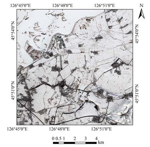
摘要: 以黑龙江省哈尔滨市道外区为研究区,系统探讨分析了基于遥感的不同方法在积雪信息识别中的应用。首先,对研究区两个时相的高分六号(GF-6)多光谱相机(PMS)影像进行目视解译,掌握了研究区内地物类型和积雪分布特点。其次,基于目视解译结果,选取了8种典型地物类型,得到了“积雪”和“非雪”两类像元的光谱特征规律。再次,探讨分析了6种方法在积雪识别中的应用,利用精确率、召回率和F指数3个指标进行了精度评价。最后,提出了基于投票结果的最终识别结果判定方法,得到了研究区积雪信息最终识别结果。研究表明:①受下垫面和阴影的影响,研究区“同谱异物”和“同物异谱”现象普遍;②深度学习算法的识别效果最好,决策树法的识别效果相对较差;农田区的识别精度高于池塘区,误识别和漏识别的现象都相对较少;③基于投票结果的最终识别结果判定,可以有效改善单一识别方法存在的误识别和漏识别现象。Abstract: From the perspective of limited research on snow recognition in high spatial resolution optical remote sensing images, considering Daowai District of Harbin City as the research area, this paper systematically discusses and analyzes the application of different methods in snow information recognition. First, ground feature types and snow distribution characteristics were mastered through visual interpretation of GF-6 PMS images of two phases in the study area. Second, based on the results of visual interpretation, eight typical surface feature types were selected, and the spectral characteristics of "snow"and "non-snow"pixels were obtained. Third, the application of the six methods in snow recognition was discussed and analyzed. Accuracy was evaluated using three indexes: positive predictive value, recall rate, and F-score. Finally, a final recognition result judgment method based on voting results was developed, and the final recognition result of snow information in the study area was obtained. The results showed that, owing to the influence of the underlying surface and shadow, the phenomenon of "same spectrum foreign matter"and "same object different spectrum"was common in the study area, which interfered with the snow recognition process to a large extent. The recognition effect of the deep learning algorithm was the best, while that of the decision tree method was relatively poor; the recognition accuracy was higher for the farmland area than that for the pond area, and the phenomenon of false and missing recognitions was relatively less. The final recognition result judgment method based on voting results can effectively improve the phenomenon of false and missing recognitions in a single recognition method. This paper has important guiding significance for snow recognition based on high-spatial-resolution optical remote sensing images.
-
Keywords:
- snow recognition /
- GF-6 PMS /
- visual interpretation /
- snow index /
- deep learning algorithm
-
0. 引言
热故障是电力设备运行时常见的一种故障类型。及时诊断出热故障,对电力设备安全运行有着重要意义。近年来,红外成像技术得到了长足的进步,运用光电技术检测物体热辐射的红外线特定波段信号,能有效显示物体表面的温度信息[1],在电力设备巡检中有着广泛应用。
随着我国电力系统的快速建设,设备红外巡检压力也愈发增大[2]。当前巡检模式严重依赖人工分析与识别。这种模式存在识别效率低、误检率和漏检率高等缺点。为此,科研人员提出多种智能化的热诊断方法。这些方法可分为如下两大类:
第一大类是基于传统图像特征的诊断方法[3-8]。一种梯度分析方法[3]应用于识别热故障目标。胡洛娜等人提出一种改进的K-均值方法[4]用于红外热故障诊断。魏钢等人提出一种基于小波变换联合后验概率分布的热故障诊断技术[5]。该方法通过改进图像质量来提高热故障诊断精度。一种粒子群图像分割[6]技术用于分割图像区域目标并进行热故障诊断。黄志鸿[8]等人采用一种低秩表示的方法,利用热故障的稀疏分布特性,将热故障从低秩背景中分离出来。第二大类是基于深度学习的诊断方法。这类方法近年来也得到广泛的关注[9-12]。魏东等人[10]利用递归神经网络定位异常热故障目标。文献[10]对红外图像进行分割,并采用卷积神经网络进行热故障识别。周可慧[11]等人提出一种改进的卷积神经网络模型,对红外热故障图像进行诊断。
文献[1]提出一种基于引导滤波的热故障诊断方法。具体来说,通过引导滤波器挖掘相邻像素间的空间结构信息,同时抑制图像中噪声等突变细节并保持热故障区域的空间边缘信息,进而提升热故障的诊断精度。然而,这项研究工作存在一个局限性,即引导滤波器的平滑程度对热故障诊断的精度影响较大。基于单一参数大小的引导滤波处理难以充分地表征红外图像复杂的空间结构信息。
为解决上述难题,本文提出一种基于多尺度引导滤波和决策融合的电力设备热故障诊断方法。该方法的主要创新点在于,联合引导滤波和多尺度决策融合技术,充分挖掘红外图像的空间结构信息和温度信息,进而提升热故障的诊断精度。该方法包括3个主要步骤。首先,基于热故障区域与图像背景在红外图像上的温度差异特性,逐像素计算热故障区域与环境背景的马氏距离,获取初始的热故障诊断结果。然后,采用不同参数设置的引导滤波对初始诊断结果进行优化,并将生成的若干引导滤波特征图堆叠在一起。最后,为充分挖掘不同尺度的引导滤波特征图的空间结构信息和温度差异信息,利用主成分分析法对引导滤波特征图进行决策融合,生成最终的热故障诊断结果图。图 1为所提出方法的流程图。
1. 引导滤波热故障诊断基本测量原理
1.1 引导滤波相关原理
图像滤波是图像处理中最常见的技术之一,其中边缘保持滤波模型近年来在机器视觉领域中有着广泛应用[13]。常见的边缘保持滤波模型有:引导滤波[13],双边滤波[14]、加权最小二乘滤波[15]。相较于其他几类边缘保持滤波技术,引导滤波采用一种简单有效的局部线性模型,具有实时性和高效性等优点[13],在图像去噪、目标检测等领域被证明为一种有效的滤波工具。具体来说,引导图像I在局部空间窗口wj中进行线性变换生成输出图像O:
$$ {O_i} = {a_j}{I_i} + {b_j},\forall i \in {w_j}, $$ (1) 式中:wj表示以像素j为中心的局部区域,空间大小为(2r+1)×(2r+1)。能量函数E(aj, bj)用于构建滤波器中系数aj和bj:
$$ {{E}}({{{a}}_{{j}}}{{,}}{{{b}}_{{j}}}) = \sum\nolimits_{{{i}} \in {{{w}}_{{j}}}} {(({{{a}}_{{j}}}{{{I}}_{{i}}}{{ + }}{{{b}}_{{j}}} - {{{p}}_{{i}}}) + \varepsilon {{{a}}_{{j}}})} $$ (2) 式中:ε为控制滤波平滑程度的参数。通过求解下列问题得到系数aj和bj:
$$ {{{a}}_{{j}}} = \frac{{\frac{1}{{\left| {{{{w}}_{{j}}}} \right|}}\sum\nolimits_{{{i}} \in {{{w}}_{{j}}}} {{{{I}}_{{i}}}{{{P}}_{{i}}} - {\mu _{{j}}}\overline {{{{P}}_{{j}}}} } }}{{{\delta _{{j}}} + \varepsilon }},{{{b}}_{{j}}}{{ = }}\overline {{{{P}}_{{j}}}} - {{{a}}_{{j}}}{\mu _{{j}}} $$ (3) 式中:P为输入的红外图像;$ \left| {{w_j}} \right| $为wj区域内的像素数;μj和δj是引导图像I中wj区域内的均值和方差;$ \overline{p_j} $是输入图像P中wj区域内均值。通过计算公式(1)生成输出图像O。
1.2 基于引导滤波的热故障诊断
在我们之前的工作中[1],提出一种基于引导滤波的热故障诊断方法。具体来说,通过引导滤波器挖掘相邻像素间的空间结构信息,同时抑制图像中噪声等突变细节并保持热故障区域的空间边缘信息,提升热故障的诊断精度。首先,根据设备故障发生区域与周围背景区域存在较大的温度差异特性,在红外图像上能较好地反映出两者的温度变化情况。由此,文献[1]中采用Reed-Xiao异常检测算法[15]来诊断出热故障区域。该算法表示如下:
$$ D_{\mathrm{RX}\left(m_i\right)}=\left(\boldsymbol{m}_i-\boldsymbol{\mu}\right) \mathit{\pmb{\Gamma}}^{-1}\left(\boldsymbol{m}_i-\boldsymbol{\mu}\right)^{\mathrm{T}} $$ (4) 式中:mi代表输入的红外图像m中的第$ i $个像素。μ和Γ分布表示为m的均值和协方差。$ {D_{RX({m_i})}} \in [0,1] $指的是第i个像素属于异常热故障的发生概率。
为提高发热故障区域的诊断精度,文献[1]对初始诊断结果图进行引导滤波处理,挖掘图像像素间的空间相似性信息,提升热故障诊断的性能。
$$F=G_{r_x, \varepsilon_x}(O, I) $$ (5) 式中:函数$ G_{r_x, \varepsilon_x}(O, I) $代表引导滤波操作;I代表输入的初始诊断结果;O指一个引导图像,它由输入红外热像的第一个主成分所组成;r和ε为两个控制滤波结果平滑度的参数。
2. 基于多尺度引导滤波和决策融合的热故障诊断方法
2.1 故障区域初始诊断
根据1.2节的工作,本文首先采用Reed-Xiao(RX)异常检测算法[16]来诊断故障区域,通过逐像素计算每一点的马氏距离,马氏距离结果为测试像素和背景像素之间的温度差异。图 2为初始诊断结果图,其右侧为初始诊断图中的两个局部放大图。初始诊断结果图像能较好地反映出异常热故障的发生区域。但未能有效去除图像中噪声等突变细节,同时丢失热故障区域部分空间边缘细节。
2.2 多尺度引导滤波特征提取
为提高热故障区域的诊断精度,不同参数大小的引导滤波器$G_{r_x, \varepsilon_x}(O, I) $对初始诊断结果图I进行特征提取:
$$ F_x=G_{r_x, \varepsilon_x}(O, I), x=1, \cdots, X $$ (6) $$F=\left\{F_1, \cdots, F_X\right\} $$ (7) 式中:rx和εx为第x组引导滤波器的两个参数,其中(rx, εx)={(r1, ε1), …, (rx, εx)}。不同滤波特征图通过公式(7)进行叠加。通过该步骤,本文所提的基于多尺度引导滤波和决策融合(multi-scale guided filter and decision fusion, MGFD)方法能够挖掘不同尺度结构信息的滤波特征图。不同参数大小的滤波特征图如图 3(b)~(e)所示。滤波后的图像有着完全不同的边缘细节和结构特征。对于含噪声的平滑区域,高平滑度可以有效降低噪声,并保持同质区域的红外光谱纯净度。因此,将这些滤波特征图叠加到一起,有助于利用不同滤波特征图的空间结构互补信息。在本文实验中(r1, ε1)=(1, 0.05),(r2, ε2)=(5, 0.1),(r3, ε3)=(10, 0.2),(r4, ε4)=(10, 0.4)。
![]() 图 3 两个滤波参数ε和r的影响:(a) 初始热故障诊断结果;(b)-(e)不同参数下的滤波特征;和(f)最终热故障诊断结果Figure 3. Influence of the two parameters, r and ε to the performance of the gulied filter: (a) Initial fault diagnosis result; (b) - (e) Filterd feature maps with different parameter settings, and (f) Finial fault diagnosis result
图 3 两个滤波参数ε和r的影响:(a) 初始热故障诊断结果;(b)-(e)不同参数下的滤波特征;和(f)最终热故障诊断结果Figure 3. Influence of the two parameters, r and ε to the performance of the gulied filter: (a) Initial fault diagnosis result; (b) - (e) Filterd feature maps with different parameter settings, and (f) Finial fault diagnosis result2.3 基于主成分分析的决策融合
在2.2节中,虽然叠加生成的高维度滤波特征图F(mn×X,m和n为图像的空间维度,X为特征图数目)能够利用图中的互补信息。然而,高维度滤波特征图F也带来了额外的数据冗余度,加重了模型的计算代价。
更重要的是,尽管引导滤波处理的目的是在保留图像同质区域的同时平滑图像边界。但值得注意的是平滑操作仍可能减少属于热故障像素和背景像素之间的光谱差异性。为解决这一难题,我们提出一种简单有效的基于主成分分析(Principal component analysis,PCA)的决策融合技术。该技术不仅可以减少数据的维数,而且能够增加像素间的光谱可分性。因此,在本文中,堆叠的滤波特征图通过PCA技术融合在一起,生成最终热故障诊断结果图:
$$P=\operatorname{PCA}(F, L) $$ (8) 式中:L为主成分的数目;F为叠加的滤波融合特征图。PCA技术将维度为mn×X的滤波特征图F,转换得到维度为mn×L的最终的热故障诊断结果图。在本文实验中,L取值1。
3. 实验分析
3.1 实验介绍
在实验中,本文采用3种经典的异常目标检测方法进行对比实验,验证所提出方法的有效性。这些方法包括基于全局统计的马氏距离计算Reed-Xiao(RX)方法[16]、低密度概率检测(low density probability,LDP)方法[17]和低秩表示(low-rank representation, LRR)[18]诊断方法。其中,对于LRR方法,参数σ设置为σ=0.05。
为评估诊断结果的优劣,本文采用线下面积(area under curve, AUC)[16, 19]指标来评估对比方法的诊断性能。该指标能较好地评估诊断结果与热故障区域的温升差异和区域面积的匹配程度,定量地评价诊断结果的精度。AUC指标越高,识别结果越接近参考的热故障区域图,热故障诊断性能越优异。
3.2 实验结果与分析
第一幅测试图像由FLIR热成像仪采集,该图像包含240×330个像素。在该图中,线路某处温度异常过热。该区域被视为热故障目标。图 4(a)和(b)展示测试图像和参考的热故障区域图。不同方法的热故障诊断结果如图 4(c)~(f)所示。在每幅图的左下方为热故障识别结果的局部放大图。如图所示,LDP和LRR方法未能有效地从背景中诊断热故障区域。相较于RX的诊断结果,MGDF的诊断结果图与参考的热故障区域图更接近。3种对比方法的AUC指标分别为0.9709、0.8312和0.8974,MGDF取得最高AUC指标,0.9985。
第二张测试图像由FLIR热成像仪所采集,该图包含240×330个像素。在该图中,线路某处的温度异常过高。该区域被视为热故障目标。图 5(c)~(f)展示了不同方法的诊断结果。RX和MGDF方法能有效地诊断出热故障区域。LDP和LRR方法不能有效去除背景像素的干扰。RX、LDP、LRR和MGDF方法的AUC标值分别为0.9901、0.9132、0.9326和0.9993。
第3幅测试图像由FILR热成像仪所采集,由325×450个像素组成。该幅图像中,绝缘子出现温度过热的异常情况。图 6(a)和(b)展示该图像的红外热图像和参考的热故障区域图。不同方法的诊断结果如图 6(c)~(f)所示。LRR方法可以诊断出热故障区域,但不能有效地去除背景像素的干扰。与RX方法的结果相比,MGDF方法最接近参考的热故障区域图。RX、LDP、LRR和MGDF方法的AUC得分分别为0.9893、0.9253、0.9486和0.9989。
不同方法AUC指标如表 1所示。如表所示,本文所提出的MGDF方法能获得最高的诊断精度(已加粗)。通过多尺度决策融合和引导滤波,MGDF相较于3种对比方法在诊断精度上有明显提升。对于3张测试图像,AUC指标分别提升0.1278,0.0601,0.0449。表 2展示了不同方法的运行时间。从表中我们可以发现,RX,LDP和LRR3种方法采用全局图像的计算策略,计算效率更高。MGDF方法需进行多尺度运算。尽管所提出的MGDF方法在运行效率上不是最高的。但鉴于其出色的诊断性能,该方法仍然是4种方法中最为实用的热故障诊断技术。
表 1 不同诊断方法的AUC指标Table 1. AUC values of different diagnosis methodsTest
imagesRX LDP LRR MGDF 1 0.9707 0.8312 0.8974 0.9852 2 0.9901 0. 9132 0. 9326 0.9993 3 0.9893 0. 9253 0. 9486 0.9989 表 2 不同诊断方法的运行时间Table 2. Running time of different diagnosis methodsTest images RX LDP LRR MGDF 1 0.59 0.75 0.47 2.31 2 0.53 0.61 0.34 2.27 3 0.84 0.98 0.56 2.15 为证明多尺度融合技术的优势,MGDF方法与基于单一尺度的引导滤波方法进行对比实验。在本文实验中,GF1、GF2、GF3、GF4分别为引导滤波参数为(r1, ε1)=(1, 0.05),(r2, ε2)=(5, 0.1),(r3, ε3)=(10, 0.2),(r4, ε4)=(10, 0.4)的滤波方法。表 3展示了不同热故障诊断方法的AUC指标值。不同滤波尺度的诊断结果有着不同的边缘细节和结构特征。本文所提的MGDF方法将这些滤波特征图叠加到一起,能够挖掘不同尺度的空间结构互补信息,进而提升热故障的诊断精度。
表 3 单一尺度滤波参数的AUC指标Table 3. Diagnosis methods with various parametersTest images GF1 GF2 GF3 GF4 MGDF 1 0.9403 0.9433 0.9681 0.9562 0.9852 2 0.9787 0.9464 0.9805 0.9908 0.9993 3 0.9693 0.9712 0.9485 0.9824 0.9989 4. 结论
在本文中,我们提出一种基于多尺度引导滤波和决策融合的电力设备热故障诊断方法。该方法的主要创新点在于,联合多尺度引导滤波和决策融合技术,充分挖掘红外图像的空间结构信息和温度信息,提升热故障的诊断精度。实验测试结果表明,本文方法在热故障诊断精度上有明显优势,满足电力设备红外巡检的应用需求满足电力红外巡检的应用需要。在未来的研究工作中,该项技术也可应用于绝缘子破损、通道树竹识别等巡检任务工作中。
-
![]()
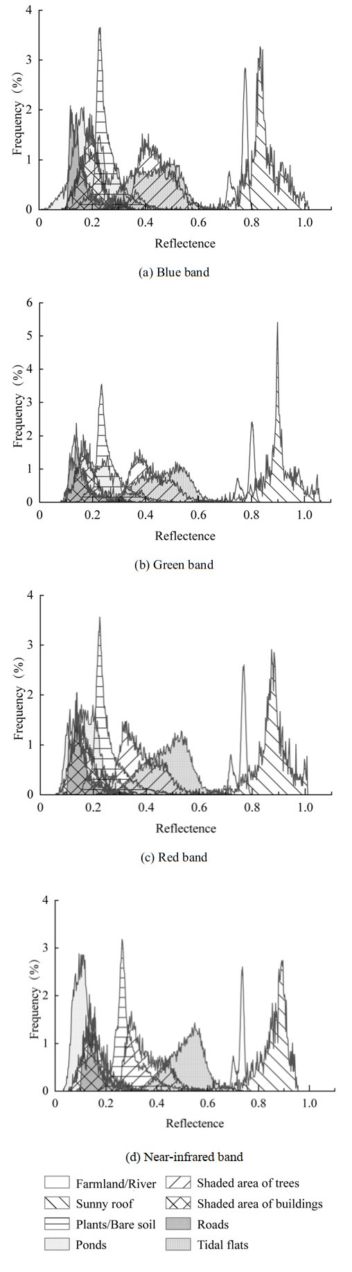
图 3 研究区典型地物波段反射率直方图
Figure 3. Histogram of reflectance of typical surface features in the study area
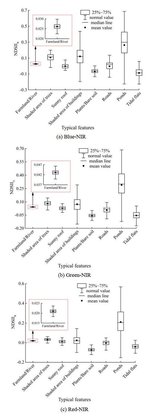
![]()
图 4 三种NDSII组合下典型地物的NDSII值
Figure 4. NDSII values of typical ground objects in three NDSII Combinations
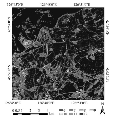
![]()
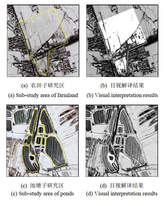
图 9 农田和池塘子研究区及目视解译结果
Figure 9. Sub-study area of farmland and ponds and corresponding visual interpretation results
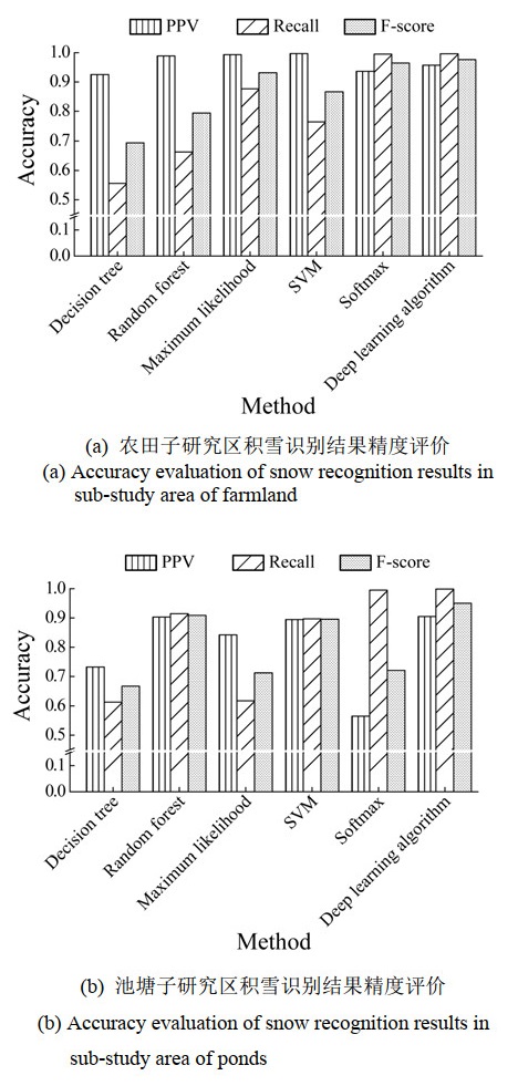
![]()
图 10 农田和池塘子研究区积雪识别结果精度评价
Figure 10. Accuracy evaluation of snow recognition results in sub-study area of farmland and ponds
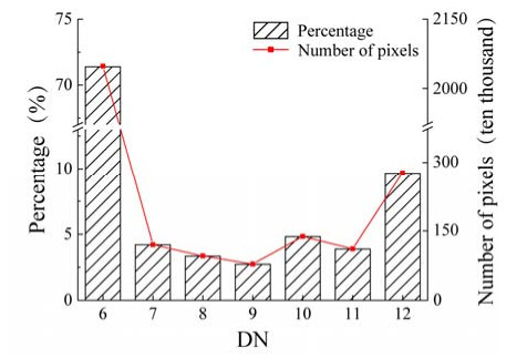
![]()
图 12 积雪识别结果叠加图像元值统计
Figure 12. DN statistics of stacking diagram of snow recognition results
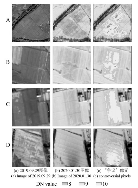
![]()
图 13 包含“争议”像元的典型农田区域
Figure 13. Typical farmland areas containing controversial pixels
![]()
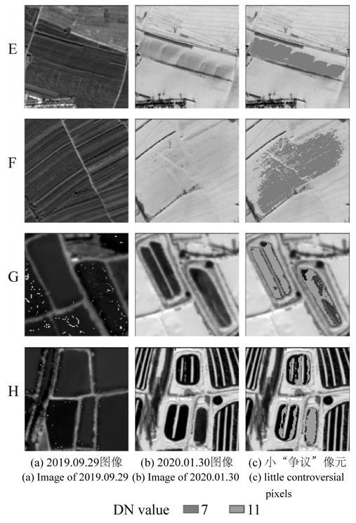
图 14 包含小“争议”像元的典型农田区域
Figure 14. Typical farmland areas containing little controversial pixels
表 1 GF-6 PMS相机参数
Table 1 Parameters of Gf-6 PMS camera
Band Spectral range/μm Spatial resolution/m Swath width/km Revisit cycle/day Blue 0.45-0.52 8 ≥90 4 Green 0.52-0.60 8 Red 0.63-0.69 8 NIR 0.76-0.90 8 Pan 0.45-0.90 2  下载: 导出CSV
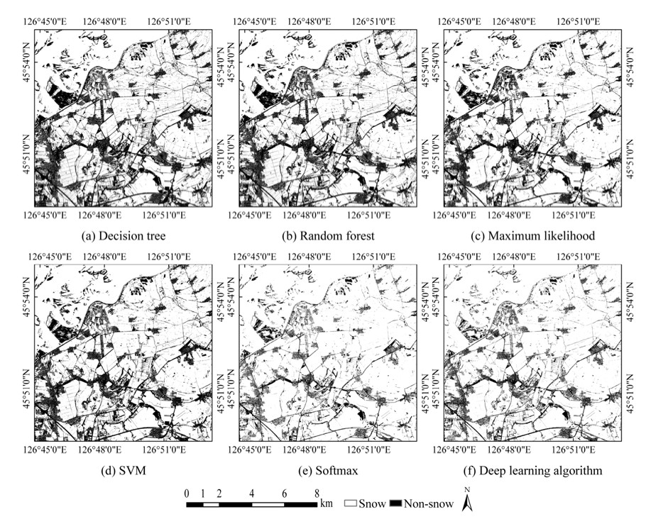
表 2 积雪识别结果统计
Table 2 Statistics of snow recognition results
Method Number of snow-covered pixels/ten thousand Ratio of snow-covered pixels/% Number of non-snow pixels/ten thousand Ratio of non-snow pixels/% Decision tree 2155.65 75.1 713.56 24.9 Random forest 2200.94 76.7 668.26 23.3 Maximum likelihood 2301.13 80.2 568.08 19.8 SVM 2239.20 78.0 630.01 22.0 Softmax 2524.23 88.0 344.98 12.0 Deep learning algorithm 2475.66 86.3 393.55 13.7
下载: 导出CSV
表 3 “争议”像元积雪识别结果统计
Table 3 Statistics of snow recognition results in controversial pixels
Area Recognition result Decision tree Random forest Maximum likelihood SVM Softmax Deep learning algorithm A Snow 0 97 5756 2196 13347 13347 Non-snow 13347 13250 7591 11151 0 0 Proportion of snow/% 0 0.7 43.1 16.5 100 100 B Snow 0 441 1078 18 2162 2162 Non-snow 2162 1721 1084 2144 0 0 Proportion of snow/% 0 20.4 49.9 0.8 100 100 C Snow 108 313 435 0 1898 1898 Non-snow 1790 1595 1463 1898 0 0 Proportion of snow/% 5.7 16.5 22.9 0 100 100 D Snow 129 316 2854 2151 3766 3765 Non-snow 3637 3450 912 1615 0 1 Proportion of snow/% 3.4 8.4 75.8 57.1 100 ≈100
下载: 导出CSV
表 4 小“争议”像元积雪识别结果统计
Table 4 Statistics of snow recognition results in little controversial pixels
Area Recognition result Decision tree Random forest Maximum likelihood SVM Softmax Deep learning algorithm E Snow 0 10115 10115 10115 10115 10115 Non-snow 10115 0 0 0 0 0 Proportion of snow/% 0 100 100 100 100 100 F Snow 0 23746 23746 23746 23746 23746 Non-snow 23746 0 0 0 0 0 Proportion of snow/% 0 100 100 100 100 100 G Snow 0 0 0 0 1169 0 Non-snow 1169 1169 1169 1169 0 1169 Proportion of non-snow/% 100 100 100 100 0 100 H Snow 19 3 0 0 1351 0 Non-snow 1354 1370 1373 1373 22 1373 Proportion of non-snow/% 98.6 99.8 100 100 1.6 100
下载: 导出CSV
-
[1] HE C, Liou K N, Takano Y, et al. Impact of grain shape and multiple black carbon internal mixing on snow albedo: Parameterization and radiative effect analysis[J]. Journal of Geophysical Research: Atmospheres, 2018, 123(2): 1253-1268. DOI: 10.1002/2017JD027752
[2] Butt M J, Bilal M. Application of snowmelt runoff model for water resource management[J]. Hydrological Processes, 2011, 25(24): 3735-3747. DOI: 10.1002/hyp.8099
[3] LIU M, XIONG C, PAN J, et al. High-resolution reconstruction of the maximum snow water equivalent based on remote sensing data in a mountainous area[J]. Remote Sensing, 2020, 12(3): 460-479. DOI: 10.3390/rs12030460
[4] XU L, Dirmeyer P. Snow–atmosphere coupling strength. Part Ⅱ: Albedo effect versus hydrological effect[J]. Journal of Hydrometeorology, 2013, 14(2): 404-418. DOI: 10.1175/JHM-D-11-0103.1
[5] 汪左. 新疆玛纳斯河流域典型区雪水当量的SAR反演研究[D]. 南京: 南京大学, 2014. WANG Zuo. Retrieval of Snow Water Equivalence Using SAR Data for Typical Area of Manas River Basin in Xinjiang, China[D]. Nanjing: Nanjing University, 2014.
[6] 贺广均. 联合SAR与光学遥感数据的山区积雪识别研究[D]. 南京: 南京大学, 2015. HE Guangjun. Snow Recognition in Mountainous Areas Based on SAR and Optical Remote Sensing Data[D]. Nanjing: Nanjing University, 2015.
[7] Barnes J C, Bowley C J. Snow cover distribution as mapped from satellite photography[J]. Water Resources Research, 1968, 4(2): 257-272. DOI: 10.1029/WR004i002p00257
[8] 冯学智. 卫星雪盖制图及其应用研究概况[J]. 遥感技术动态, 1989(1): 25-29. https://www.cnki.com.cn/Article/CJFDTOTAL-YGJS198901004.htm FENG Xuezhi. Satellite snow cover mapping and its application[J]. Development of Remote Sensing Technology, 1989(1): 25-29. https://www.cnki.com.cn/Article/CJFDTOTAL-YGJS198901004.htm
[9] 冯学智. 卫星雪盖制图中的一些技术问题[J]. 遥感技术与应用, 1991(4): 10-15. https://www.cnki.com.cn/Article/CJFDTOTAL-YGJS199104001.htm FENG Xuezhi. Some technical problems in satellite snowcover mapping[J]. Remote Sensing Technology and Application, 1991(4): 10-15. https://www.cnki.com.cn/Article/CJFDTOTAL-YGJS199104001.htm
[10] 白磊, 郭玲鹏, 马杰, 等. 基于数字相机拍摄影像的山区积雪消融动态观测研究——以天山积雪站为例[J]. 资源科学, 2012, 34(4): 620-628. https://www.cnki.com.cn/Article/CJFDTOTAL-ZRZY201204006.htm BAI Lei, GUO Lingpeng, MA Jie, et al. Observation and analysis of the process of snow melting at Tianshan station using the images by digital camera[J]. Resouces Science, 2012, 34(4): 620-628. https://www.cnki.com.cn/Article/CJFDTOTAL-ZRZY201204006.htm
[11] Kim S-H, Hong C-H. Antarctic land-cover classification using IKONOS and Hyperion data at Terra Nova Bay[J]. International Journal of Remote Sensing, 2012, 33(22): 7151-7164. DOI: 10.1080/01431161.2012.700136
[12] ZHU L, XIAO P, FENG X, et al. Support vector machine-based decision tree for snow cover extraction in mountain areas using high spatial resolution remote sensing image[J]. Journal of Applied Remote Sensing, 2014, 8(1): 084698. DOI: 10.1117/1.JRS.8.084698
[13] Dozier J. Spectral signature of alpine snow cover from the Landsat Thematic Mapper[J]. Remote Sensing of Environment, 1989, 28(1): 9-22. http://static1.1.sqspcdn.com/static/f/891472/15152129/1321451632750/Dozier_J._1989.pdf?token=sMvVhVmXaLvHsiAGq%2FlmCvgkjlA%3D
[14] Cea C, Cristóbal J, Pons X. An improved methodology to map snow cover by means of Landsat and MODIS imagery[C]//2007 IEEE International Geoscience and Remote Sensing Symposium, 2007: 4217-4220.
[15] Khosla D, Sharma J, Mishra V. Snow cover monitoring using different algorithm on AWiFS sensor data[J]. International Journal of Advanced Engineering Sciences and Technologies, 2011, 7(1): 42-47.
[16] 延昊. 利用MODIS和AMSR-E进行积雪制图的比较分析[J]. 冰川冻土, 2005(4): 515-519. DOI: 10.3969/j.issn.1000-0240.2005.04.008 YAN Hao. A comparison of MODIS and passive microwave snow mapping[J]. Journal of Glaciology and Geocryology, 2005(4): 515-519. DOI: 10.3969/j.issn.1000-0240.2005.04.008
[17] 郝晓华, 王建, 李弘毅. MODIS雪盖制图中NDSI阈值的检验——以祁连山中部山区为例[J]. 冰川冻土, 2008(1): 132-138. https://www.cnki.com.cn/Article/CJFDTOTAL-BCDT200801020.htm HAO Xiaohua, WANG Jian, LI Hongyi. Evaluation of the NDSI threshold value in mapping snow cover of MODIS[J]. Journal of Glaciology and Geocryology, 2008(1): 132-138. https://www.cnki.com.cn/Article/CJFDTOTAL-BCDT200801020.htm
[18] 汪凌霄. 玛纳斯河流域山区积雪遥感识别研究[D]. 南京: 南京大学, 2012. WANG Lingxiao. Retrieval of Snow Water Equivalence Using SAR Data for Typical Area of Manas River Basin in Xinjiang, China[D]. Nanjing: Nanjing University, 2012.
[19] Baghdadi N, Gauthier Y, Bernier M. Capability of multitemporal ERS-1 SAR data for wet-snow mapping[J]. Remote Sensing of Environment, 1997, 60(2): 174-186. DOI: 10.1016/S0034-4257(96)00180-0
[20] Rott H, Nagler T. Capabilities of ERS-1 SAR for snow and glacier monitoring in alpine areas[J]. European Space Agency-Publications-ESA SP, 1994, 361: 965-965. http://www.researchgate.net/publication/245605630_Capabilities_of_ERS-1SAR_for_snow_and_glacier_monitoring_in_Alpine_areas
[21] Koskinen J T, Pulliainen J T, Hallikainen M T. The use of ERS-1 SAR data in snow melt monitoring[J]. IEEE Transactions on Geoscience Remote Sensing, 1997, 35(3): 601-610. DOI: 10.1109/36.581975
[22] Luojus K P, Pulliainen J T, Cutrona A B, et al. Comparison of SAR-based snow-covered area estimation methods for the boreal forest zone[J]. IEEE Geoscience Remote Sensing Letters, 2009, 6(3): 403-407. DOI: 10.1109/LGRS.2009.2014786
[23] Caves R, Hodson A, Turpin O, et al. Field verification of SAR wet snow mapping in a non-Alpine environment[J]. European Space Agency- Publications- ESA SP, 1998, 441: 519-526. http://www.researchgate.net/publication/228650728_Field_verification_of_SAR_wet_snow_mapping_in_a_non-Alpine_environment/download
[24] Malnes E, Guneriussen T. Mapping of snow covered area with Radarsat in Norway[C]//IEEE International Geoscience and Remote Sensing Symposium, 2002: 683-685.
[25] Kelly R. The AMSR-E snow depth algorithm: description and initial results[J]. Journal of the Remote Sensing Society of Japan, 2009, 29(1): 307-317. https://www.jstage.jst.go.jp/article/rssj/29/1/29_1_307/_pdf/-char/en
[26] PAN J, JIANG L, ZHANG L. Wet snow detection in the south of China by passive microwave remote sensing[C]//IEEE International Geoscience and Remote Sensing Symposium, 2012: 4863-4866.
[27] Singh P R, Gan T Y. Retrieval of snow water equivalent using passive microwave brightness temperature data[J]. Remote Sensing of Environment, 2000, 74(2): 275-286. DOI: 10.1016/S0034-4257(00)00121-8
[28] LIU X, JIANG L, WU S, et al. Assessment of methods for passive microwave snow cover mapping using FY-3C/MWRI data in China[J]. Remote Sensing, 2018, 10(4): 524-545. DOI: 10.3390/rs10040524
[29] Hinkler J, Pedersen S B, Rasch M, et al. Automatic snow cover monitoring at high temporal and spatial resolution, using images taken by a standard digital camera[J]. International Journal of Remote Sensing, 2002, 23(21): 4669-4682. DOI: 10.1080/01431160110113881
[30] Keshri A, Shukla A, Gupta R. ASTER ratio indices for supraglacial terrain mapping[J]. International Journal of Remote Sensing, 2009, 30(2): 519-524. DOI: 10.1080/01431160802385459
[31] Hinkler J, Ørbæk J B, Hansen B. Detection of spatial, temporal, and spectral surface changes in the Ny-Ålesund area 79 N, Svalbard, using a low cost multispectral camera in combination with spectroradiometer measurements[J]. Physics Chemistry of the Earth, Parts A/B/C, 2003, 28(28-32): 1229-1239. DOI: 10.1016/j.pce.2003.08.059
[32] XIAO X M, SHEN Z X, QIN X G. Assessing the potential of VEGETATION sensor data for mapping snow and ice cover: a normalized difference snow and ice index[J]. International Journal of Remote Sensing, 2001, 22(13): 2479-2487. DOI: 10.1080/01431160119766
[33] XIAO X, Moore B, QIN X, et al. Large-scale observations of alpine snow and ice cover in Asia: using multi-temporal vgetation sensor data[J]. International Journal of Remote Sensing, 2002, 23(11): 2213-2228. DOI: 10.1080/01431160110076180
[34] Long J, Shelhamer E, Darrell T. Fully convolutional networks for semantic segmentation[C]//Proceedings of the IEEE Conference on Computer Vision and Pattern Recognition, 2015: 3431-3440.
-
期刊类型引用(2)
1. 黄坤琳,吴国周,徐维新,李利东,王海梅,李航,李自翔,司荆柯,刘洪宾,吴成娜. 呼伦贝尔东部农田区动态融雪过程及其影响因子. 干旱区研究. 2024(09): 1514-1526 .  百度学术
百度学术
2. 黄林,李晖,康璇. 基于Freeman全极化分解的干雪识别指数模型构建. 厦门理工学院学报. 2023(05): 40-48 . 百度学术
其他类型引用(2)


计量
- 文章访问数: 367
- HTML全文浏览量: 95
- PDF下载量: 42
- 被引次数: 4
